CONN

ROI-to-ROI analysis with the CONN toolbox

Following the standard preprocessing pipeline, the CONN toolbox (Nieto-Castanon 2020) takes care of the FC generation after denoising. This is an add-on to SPM that can be downloaded here.

STEP 1. Importing the data into a new CONN project

This script will create a new conn project named conn_example and automatically import the functional and structural volumes for the set number of subjects.

% Created by Andrew Jahn, University of Michigan, 02.27.2020
% Adapted by Clément Guichet, UGA, LPNC, 07.01.2023

% FIND functional/structural files
NSUBJECTS= X;
cwd=pwd;

# the smoothed out spatially preprocessed volumes, conn will automatically bind them to the unsmoothed ones
FUNCTIONAL_FILE=cellstr(conn_dir('swar*.nii'));
STRUCTURAL_FILE=cellstr(conn_dir('wm*.nii'));
if rem(length(FUNCTIONAL_FILE),NSUBJECTS),error('mismatch number of functional files %n', length(FUNCTIONAL_FILE));end
if rem(length(STRUCTURAL_FILE),NSUBJECTS),error('mismatch number of anatomical files %n', length(FUNCTIONAL_FILE));end
nsessions=length(FUNCTIONAL_FILE)/NSUBJECTS;
FUNCTIONAL_FILE=reshape(FUNCTIONAL_FILE,[nsessions, NSUBJECTS]);
STRUCTURAL_FILE={STRUCTURAL_FILE{1:NSUBJECTS}};
disp([num2str(size(FUNCTIONAL_FILE,1)),' sessions']);
disp([num2str(size(FUNCTIONAL_FILE,2)),' subjects']);
TR= X; % Repetition time


% CONN-SPECIFIC SECTION: RUNS SETUP STEPS
% Prepares batch structure
clear batch;
batch.filename=fullfile(cwd,'conn_example.mat'); % New conn_*.mat experiment name

% SETUP step
batch.Setup.isnew=1;
batch.Setup.nsubjects=NSUBJECTS;
batch.Setup.RT=TR; % TR (seconds)

batch.Setup.functionals=repmat({{}},[NSUBJECTS,1]); % Pre-allocation
% Point to functional volumes for each subject/session
for nsub=1:NSUBJECTS
    for nses=1:nsessions
        batch.Setup.functionals{nsub}{nses}{1}=FUNCTIONAL_FILE{nses,nsub};
    end
end 
batch.Setup.structurals=STRUCTURAL_FILE; % Point to anatomical volumes for each subject


% Define the names and files for the covariates
covariate_names = {'Art_outliers_&_movement'};
ART_FILE = cellstr(conn_dir('art_regression_outliers_and_movement_warRS.mat'));
ncovariate=length(ART_FILE)/NSUBJECTS;
ART_FILE = reshape(ART_FILE, [ncovariate, NSUBJECTS]);
disp([num2str(size(ART_FILE,1)),'covariate']);
disp([num2str(size(ART_FILE,2)),'subjects']);

% Add covariates
batch.Setup.covariates.add=1;
batch.Setup.covariates.names=covariate_names; 
for ncov=1:ncovariate
    for nsub=1:NSUBJECTS
        for nses=1:nsessions
            batch.Setup.covariates.files{ncov}{nsub}{nses}{1}=ART_FILE{nses,nsub,ncov}; 
        end 
    end
end


% Run all analyses
conn_batch(batch);

STEP 2. Running CONN in the GUI

After creating the project, you can open the gui by typing:

conn
conn('load', fullfile(cwd, 'conn_example.mat'))

If the project does not load up, you can open the mat file in the GUI.

Atlas selection & Denoising

1. Check that the structural and functional volumes have all been imported correctly.

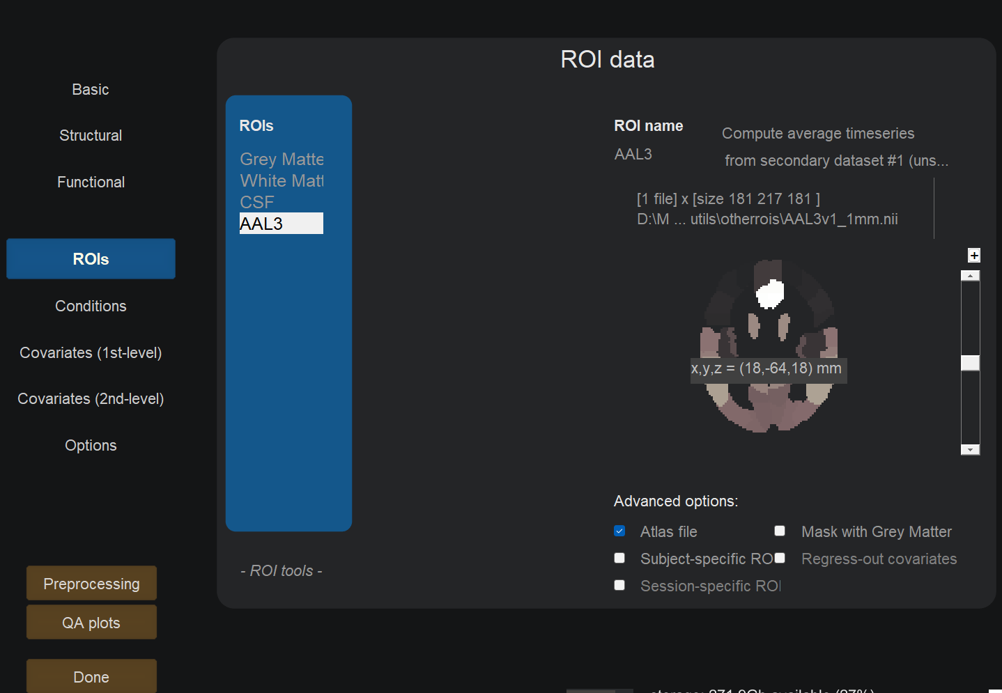
2. In the ROIs field, remove the default atlas if there is one and import yours in NIFTI format.

3. Check the ‘Atlas file’ box.

   

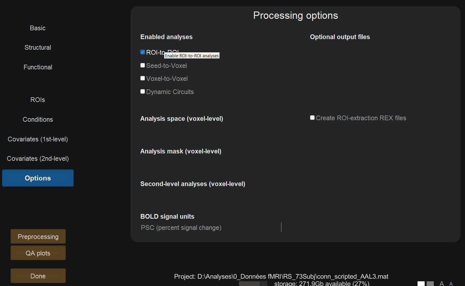
4. In the Options field, enable ROI-to-ROI analyses only.

   

5. Click done. This may take up a few hours depending on the cohort size.

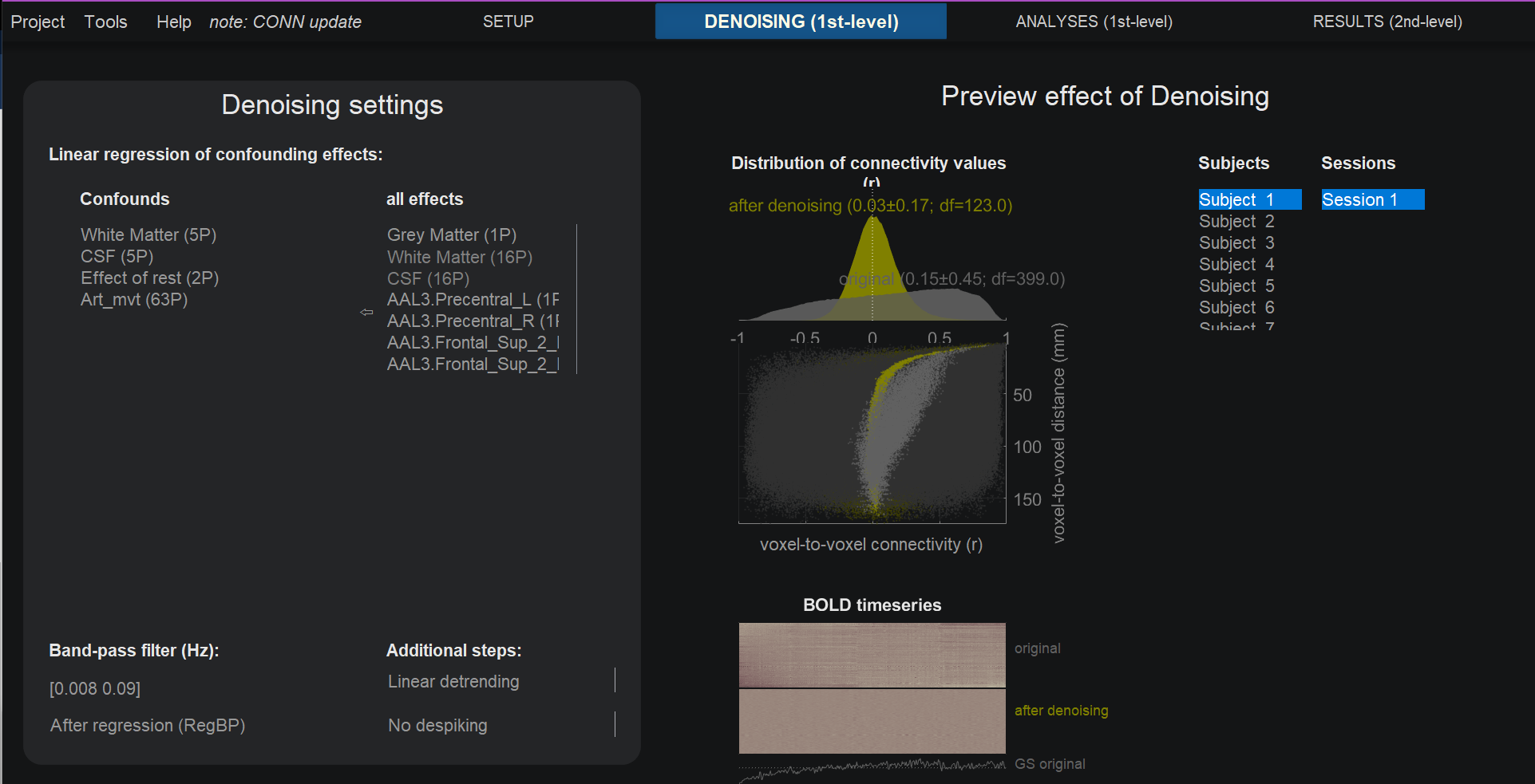
6. By default, CONN includes regressors derived from the tissue types you generated in the ROIs section (WM, CSF) of the Setup tab, and the 1st-level covariates of the Setup tab (Art_mvt). You can leave the default settings and proceed to the 1st-level analyses by clicking done.

   

Generate the Functional Connectome (FC)

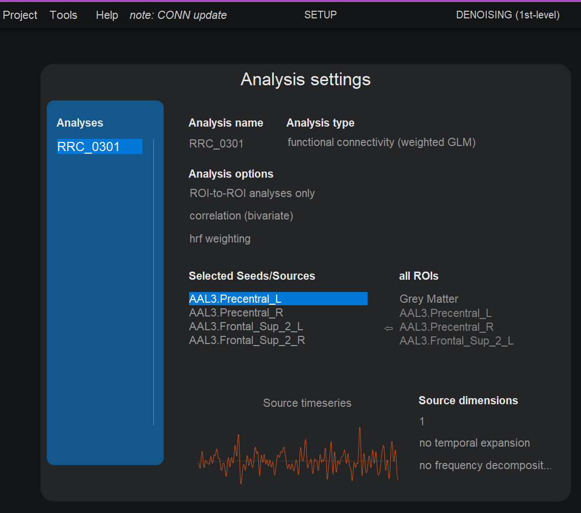
1. Create a new analysis and select RRC (ROI-to-ROI connectivity).

2. Select the brain regions to be included in the connectome.

   

3. Click done to generate the .mat file. Under the path /conn_example/results/firstlevel/RRC, you should now visualize the .mat files for each subject.

   

References

Nieto-Castanon, Alfonso. 2020. Handbook of Functional Connectivity Magnetic Resonance Imaging Methods in CONN. Hilbert Press. https://doi.org/10.56441/hilbertpress.2207.6598.